Population estimates
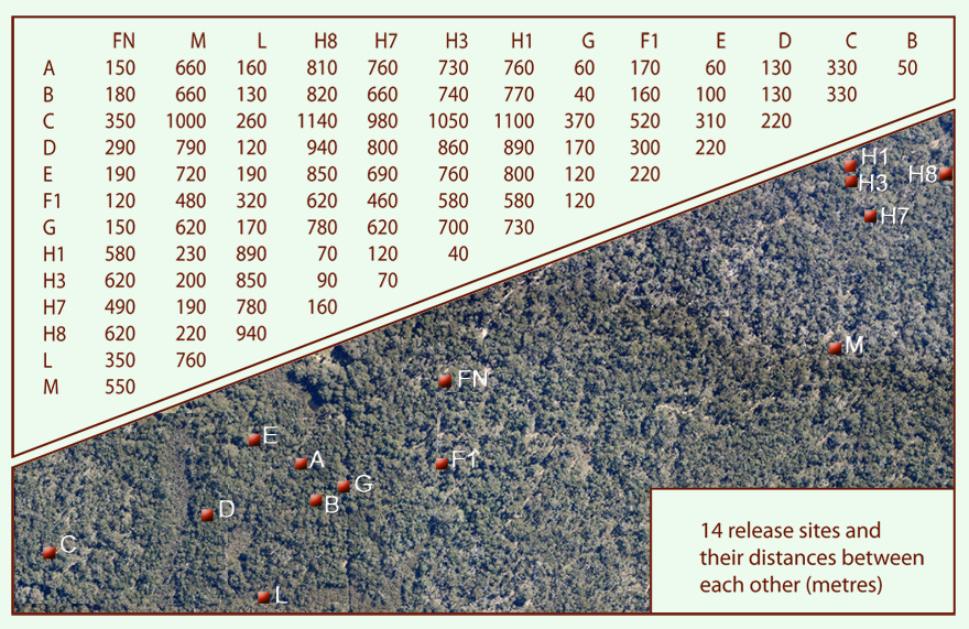
In June 2012 we started releasing a number of Western Ringtail Possums at what is now our major release site with 14 different spots.
The sites are named alphabetically. The same letter indicates the same release date but not necessarily the same spot. The numbers of cages are added in brackets:
A(4), B(2), C(4), D(3), E(7), F1(3), G(5), H1(2), H3(2), H7(3), H8(2), L(3) , M(2) and FN(1) (see image).
Each release is documented photographically with night vision cameras. With increasing numbers of available cameras we were able to have a separate camera for every release cage as early as from release C.
Where cages had to be shifted to an upcoming release site, the camera had to go with it. The previous, left vacant site was not monitored anymore.
Those sites came back into our observation when at the beginning of summer 2014 we installed water stations at all those temporarily vacant places and added a camera each.
At this point of time all the above listed sites were equipped to be monitored around the clock.
To estimate the number of ringtails at a particular time at all release spots we used a spreadsheet detailing the 14 sites and 52 time-collumns representing 13 hours (52 quarters) from 5pm to 6am.
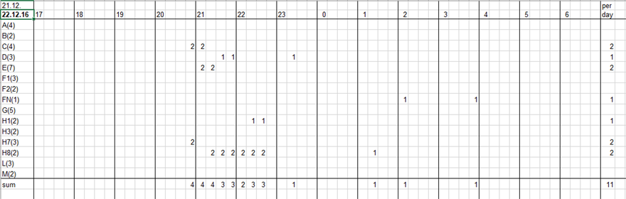
If a minimum of one ringtail-photo per quarter was triggered at any site the number of ringtails on this image was registered. If several photos were triggered in the same intervall only the highest number of ringtails was listed once.
Therefore, the number noted during a 15 minutes period at any release site is the lowest figure of confirmed animals.
However, as the densities in mixed habitat are generally low, a 15 minute intervall is far too short for a reliable count. Also, animals mainly approach our monitoring spots when in need of water. At other times they would stay outside the monitored area.
As ringtail possums are territorial, we assumed that extending the time frame to one day would not lead to double-counts if again only the highest number of animals that are shown together on one photo are taken into consideration. The monitoring spots are far enough apart to minimise the risk that animals travel from one to the other during that one day and the limited number of monitoring spots would counter-balance any (still possible) double counts. A number of animals will presumably not be noted by any of the cameras. Adding up the noted sighting at all spots in one day would produce a minimum number of ringtails alive on the property at a particular day.
Further considerations aimed at estimating the size of the population to be able to notice any future trends. We therefore relied upon the lower number of definitely present animals instead of a possibly more acurate figure through additional analysis of the photos and comparison of morphological features.
We are unaware of any formula for estimates based on camera monitoring and had to use one that seemed most appropriate which was Magnusson, Caughley und Grigg, ’A double-survey estimate of population size from incomplete counts’ which was published in 1978. (Magnusson et al, 1978)
Two counts/rows of figures are necessary which do not necessarily have to be generated through a survey by a person and which do not need to be sequential. Not even the methods used to generate the two lines of figures has to be identical.
B = Number of animals seen at the same spot in both counts
S1 = Number of animals seen only in the first count, not the second
S2 = Number of animals seen only in the second count, not the first
M = unkown figure of animals, missed in both counts
N = estimated population size
P1 = probability of ringtail sightings in count one
P2 = probability of ringtail sightings in count two
N and M are unkown and therefore 2 formulae are required
First equation:
The sum of the known figures B plus S1 plus S2 plus the unkown figure M of missed animals equals N:
(1) N = B + S1 + S2 + M
Second equation:
Probability for B equals P1*P2
Probability for S1 equals P1(1-P2)
Probability for S2 equals P2(1-P1)
Probability for M equals (1-P1)*(1-P2)
The sum of those probabilities equals 1
(2) 1 = P1*P2 + P1(1-P2) + P2(1-P1) + (1-P1)(1-P2)
The unknown parameters can be estimated on the basis of the known parameters (B, S1 and S2).
Based on the Lincoln-Petersen estimate and corrected by Chapman (1951):


As shown above we define a ‚day‘ as: the 13 nightly hours between 5 pm yesterday evening and 6 am today. It is registered under today‘s date.
Based on this we have estimated N (3), P1 (4) and P2 (5) for every single day since we started to release in May 2012. The follwing example shows one month.

Equation (3) shows the minimum number of ringtails estimated for one day.
One day is a short time span and if the sum of S1+S2+2B is smaller than N, there is bias. This has happened several times in our calculations - marked in red - and those had to be excluded. Bias was strongest in December 2016 counts and we hypothesize that the reduced reliability of the digital cameras in hot weather has led to the problem. If considering 2 days pooling instead of just 1 bias is removed.
Used terms are defined as following:
Cell = one field of a table or spreadsheet which is the junction between a row (horizontal) and a column (vertical)
Marked cell = is a cell showing any number of ringtail sightings
Total cells = all available cells (here number of days multiplied by number of sites)
% of marked cells = percentage of number of all marked cells
V = Value of one cell (or the average of several cells) showing the number of simultaneously present ringtails - (ringtails divided by marked cells). This would be equal or smaller than 3 (including decimals)
P = the average of P1 and P2 for the whole table
Nmax = the highest estimated population number N of the whole table
Pmax = the average probability
P1 and P2 only for the date of Nmax.
For the period from 13.08. to 30.12. 2016 the following results were registered for our usual 14 sites. (see first row of table below)
To reduce the risk of double counts because of ringtails moving around, we combined those sites that were close to each other – in one case just two of them (H1 and H3) but in the second case we combined four (A,B,E and G). The results are listed in the second row (11 sites).
total cells |
marked cells |
ringtails |
Nmax |
value |
marked of total |
P |
biased |
|
14 sites |
1960 |
788 |
1101 |
27 |
1.4 |
40.2 % |
60% |
25 |
11 sites |
1540 |
663 |
965 |
19 |
1.45 |
43% |
62% |
12 |
These two rows represent the very same counts and sightings at the very same time - apart from the number of sites. When comparing the results, 136 ringtails less were counted for 11 sites and Nmax was lower by 8. This figures seemed too high to account for double counts as there are fire breaks between A/ E and B and G. Animals seem to rarely cross those breaks.
As mentioned earlier, monitoring data are available on a daily base from the beginning of our releases.
For comparison reasons our yearly data collection tables (until 2018) have the same size - 14 rows (sites) and 365/366 columns (days) even though in the early phase some sites were not established let alone monitored yet (e.g. sites L and M only established in 2015). Also, the table stayed undiminished during maintenance or if cameras were dysfunctional. We updated this from 2019 (see below).
'Double-survey estimates of population size from incomplete counts' are used on a daily base. Each set of data of two adjasent days are used as a single survey, either complete or fragmental. The results show the whole spectrum of quality from 'excellent' to 'very poor' whith some biased because of the lack of data. But the trends are obvious.
total cells |
marked cells |
ringtails |
Nmax |
value |
marked of total |
P |
Pmax |
biased | |
2015 |
5110 |
1648 |
2326 |
22 |
1.4 |
32% |
58% |
47% |
61 |
2016 |
5124 |
1962 |
2606 |
27 |
1.3 |
38% |
59% |
43% |
59 |
2017 |
5110 |
2685 |
3691 |
31 |
1.35 |
52.5% |
65% |
50% |
34 |
2018 |
5110 |
2898 |
3752 |
27 |
1.3 |
56.7% |
60% |
53% |
41 |
2019 |
5760 |
3168 |
4066 |
32 |
1.3 |
55.0% |
64% |
56% |
39 |
| 2020 | 5776 | 3435 | 4844 | 39 | 1.4 | 59.0% | 65.4% | 66.8% | 42 |
| 2021 | 5840 | 2921 | 3971 | 31 | 1.4 | 50% | 66.6% | 68.3% | 67 |
Pooling might help to find a factor (f) to be multiplied with the ‚estimated population size‘ to come as close as possible to the true number of ringtails present. It will increase both, the number of marked cells and the average value of those cells simultaneously.
Actually we have pooled already when we selected the image with the highest number of ringtails per 15 minute interval. When we combined all the 15 minute periods into 13 hours or 1 day, we basically pooled again.
We have used the same pooling conditions and data for the years 2015 until 2020: the last 15 weeks of the year from (18 September until 31 December for instance; there are just 7 2-weeks periods and the last of the 4-weeks period has just 3 weeks).
Starting with one week (or 7 days) the time period was increased in steps to 5 weeks (or 35 days). Only the highest number of simultaneously present animals again was used in those tables.
We looked at:
15 1-week periods, see following pool tables (collumn A)
7 2-weeks periods, see following pool tables (collumn B)
5 3-weeks periods, see following pool tables (collumn C)
4 4-weeks periods, see following pool tables (collumn D)
3 5-weeks periods, see following pool tables (collumn E)
Unpooled daily data, can be found at collumn X of each year's table.
| 2015 | X |
A |
B |
C |
D |
E |
| Total cells | 1456 |
210 |
98 |
70 |
56 |
42 |
| Marked cells | 472 |
119 |
62 |
52 |
41 |
33 |
| Seen ringtails | 747 |
224 |
119 |
105 |
83 |
68 |
| Marked cells value | 1.6 |
1.9 |
1.9 |
2 |
2 |
2.1 |
| Value differences A,B,C,D,E to X | 0.3 |
03 |
0.4 |
0.4 |
0.5 |
|
| % of value differences (3 ringtails per cell = 100%) | 10% |
10% |
13% |
13% |
17% |
|
| % of 'marked cells of total cells' | 32% |
57% |
63% |
74% |
73% |
79% |
| Geometrical sum of '% of value difference' and '% of marked cells' |
58% |
63% |
75% |
74% |
81% |
|
| % of geometrical sums A,B,C,D,E divided by % X - equals factor (f) | 1.8 |
2 |
2.3 |
2.3 |
2.5 |
| 2016 | X |
A |
B |
C |
D |
E |
| Total cells | 1456 |
210 |
98 |
70 |
56 |
42 |
| Marked cells | 603 |
168 |
86 |
64 |
50 |
39 |
| Seen ringtails | 871 |
287 |
161 |
126 |
103 |
82 |
| Marked cells value | 1.4 |
1.7 |
1.9 |
2 |
2.1 |
2.1 |
| Value differences A,B,C,D,E to X | 0.3 |
0.5 |
0.6 |
0.7 |
0.7 |
|
| % of value differences (3 ringtails per cell = 100%) | 10% |
17% |
20% |
23% |
23% |
|
| % of 'marked cells of total cells' | 38% |
80% |
88% |
91% |
89% |
93% |
| Geometrical sum of '% of value difference' and '% of marked cells' |
81% |
90% |
93% |
92% |
96% |
|
| % of geometrical sums A,B,C,D,E divided by % X - equals factor (f) | 2.1 |
2.4 |
2.4 |
2.4 |
2.5 |
| 2017 | X |
A |
B |
C |
D |
E |
| Total cells | 1456 |
210 |
98 |
70 |
56 |
42 |
| Marked cells | 785 |
175 |
85 |
63 |
51 |
39 |
| Seen ringtails | 1181 |
340 |
184 |
138 |
114 |
89 |
| Marked cells value | 1.5 |
1.9 |
2.2 |
2.2 |
2.2 |
2.3 |
| Value differences A,B,C,D,E to X | 0.4 |
0.7 |
0.7 |
0.7 |
0.8 |
|
| % of value differences (3 ringtails per cell = 100%) | 13% |
23% |
23% |
23% |
27% |
|
| % of 'marked cells of total cells' | 52.5% |
83% |
87% |
90% |
91% |
93% |
| Geometrical sum of '% of value difference' and '% of marked cells' |
84% |
90% |
93% |
94% |
97% |
|
| % of geometrical sums A,B,C,D,E divided by % X - equals factor (f) | 1.6 |
1.7 |
1.8 |
1.8 |
1.8 |
| 2018 | X |
A |
B |
C |
D |
E |
| Total cells | 1456 |
210 |
112 |
70 |
56 |
42 |
| Marked cells | 840 |
199 |
107 |
70 |
56 |
42 |
| Seen ringtails | 1135 |
348 |
201 |
140 |
113 |
94 |
| Marked cells value | 1.35 |
1.7 |
1.9 |
2 |
2 |
2.2 |
| Value differences A,B,C,D,E to X | 0.35 |
0.55 |
0.65 |
0.65 |
0.85 |
|
| % of value differences (3 ringtails per cell = 100%) | 12% |
18% |
22% |
22% |
28% |
|
| % of 'marked cells of total cells' | 56.7% |
95% |
96% |
100% |
100% |
100% |
| Geometrical sum of '% of value difference' and '% of marked cells' | 96% |
97% |
102% |
102% |
104% |
|
| % of geometrical sums A,B,C,D,E divided by % X - equals factor (f) | 1.7 |
1.7 |
1.8 |
1.8 |
1.8 |
Each of the last table rows represents the 'faktor (f)' we were looking for.
Utilising the factor '2', we estimate at least '34' western ringtail possums on the property in 2014, up to '44' in 2015, in access of '54' in 2016, less than '62' in 2017 and 54 again in 2018.
There is another approach to find similar numbers using the ‘seeing-a-ringtail-probability Pmax‘, which is the average of P1 and P2 regarding to the date with the most of seen ringtails 'Nmax'. In 2015 Nmax equals 22 where Pmax equals 47 %. 100 % of ‘seeing-a-ringtail-probability P‘equals 100*Nmax/Pmax or '47' ringtails in 2015, '63' in 2016, '62' in 2017 and '51' in 2018.
Things have changed in 2019.
Two more Western Ringtail Possums were released and monitored ('N' two Cameras) since April.
Another
waterer was installed elsewhere and monitored ('FE' one camera ) in April as well. (See 2019 pool table below, 'Total cells' etc. in collumns X.)

| 2019 | X |
A |
B |
C |
D |
E |
| Total cells | 1680 |
240 |
128 |
80 |
64 |
48 |
| Marked cells | 936 |
225 |
128 |
80 |
64 |
48 |
| Seen ringtails | 1312 |
390 |
243 |
162 |
135 |
101 |
| Marked cells value | 1.3 |
1.7 |
1.9 |
2 |
2.1 |
2..1 |
| Value differences A,B,C,D,E to X | 0.4 |
0.6 |
0.7 |
0.8 |
0.8 |
|
| % of value differences (3 ringtails per cell = 100%) | 13.3% |
20% |
23.3% |
26.7% |
26.7% |
|
| % of 'marked cells of total cells' | 55.0% |
94% |
100% |
100% |
100% |
100% |
| Geometrical sum of '% of value difference' and '% of marked cells' | 94.3% |
102% |
102.7% |
103% |
103% |
|
| % of geometrical sums A,B,C,D,E divided by % X - equals factor (f) | 1.7 |
1.85 |
1.87 |
1.87 |
1.87 |
Utilising a factor '1.9' the population estimate equals '61' Western Ringtail Possums in 2019.
The 100% probability for 2019 would equal '50' Western Ringtail Possums at this site.
The monitoring stations in 2020 are the same as in 2019:
| 2020 | X |
A |
B |
C |
D |
E |
| Total cells | 1680 |
240 |
128 |
80 |
64 |
48 |
| Marked cells | 925 |
226 |
124 |
79 |
64 |
48 |
| Seen ringtails | 1384 |
396 |
228 |
153 |
127 |
100 |
| Marked cells value | 1.5 |
1.8 |
1.8 |
1.9 |
2.0 |
2.1 |
| Value differences A,B,C,D,E to X | 0.3 |
0.3 |
0.4 |
0.5 |
0.6 |
|
| % of value differences (3 ringtails per cell = 100%) | 10% |
10% |
13.3% |
16.7% |
20% |
|
| % of 'marked cells of total cells' | 59.0% |
94% |
96.9% |
98.8% |
100% |
100% |
| Geometrical sum of '% of value difference' and '% of marked cells' | 94.5% |
97.4% |
99.7% |
101.3% |
102% |
|
| % of geometrical sums A,B,C,D,E divided by % X - equals factor (f) | 1.6 |
1.65 |
1.7 |
1.71 |
1.73 |
Utilising a factor '1.7' the population estimate equals '66' Western Ringtail Possums in 2020.
The 100% probability for 2020 would equal '60' Western Ringtail Possums at this site.
The monitoring stations in 2021 are the same as in 2019, but this time using the whole year's data, not only those of the last 15 weeks:
| 2021 | X |
A |
B |
C |
D |
E |
| Total cells | 5840 |
832 |
416 |
272 |
208 |
160 |
| Marked cells | 2921 |
738 |
402 |
268 |
205 |
159 |
| Seen ringtails | 3971 |
871 |
588 |
482 |
381 |
302 |
| Marked cells value | 1.4 |
1.18 |
1.46 |
1.8 |
1.86 |
1.9 |
| Value differences A,B,C,D,E to X | (-)0.2 |
0.06 |
0.4 |
0.46 |
0.5 |
|
| % of value differences (3 ringtails per cell = 100%) | negat. |
0.2% |
13.3% |
15.3% |
16.7% |
|
| % of 'marked cells of total cells' | 50% |
(-)89% |
97% |
98.5% |
98.6% |
100% |
| Geometrical sum of '% of value difference' and '% of marked cells' | 97.4% |
99.4% |
99.8% |
100% |
||
| % of geometrical sums A,B,C,D,E divided by % X - equals factor (f) | 1.9 |
2 |
2 |
2 |
In 2021 we have found a factor of 2. The unbiased estimation of Nmax was 31. As a result the Western Ringtail Possum population could well have been 62.
The probability tells exactly the same.
![]()